Exploring the Structure of Operational Amplifiers
Some engineers emphasize the infinite gain of an ideal operational amplifier, focusing on virtual open and virtual short circuits when analyzing op-amps, while neglecting some more important concepts such as common-mode rejection ratio, offset voltage, and bias current
1. Operational Amplifier Input Model
Based on the operational amplifier model, a comprehensive overview of the basic op-amp model can be summarized as follows: it is the superposition of differential-mode and common-mode signals.

2. Virtual Short Circuit Concept
For an ideal operational amplifier, it's important to understand the concepts of virtual open circuit and virtual short circuit. The non-inverting input and inverting input of the operational amplifier are equal.

An ideal operational amplifier has infinite open-loop gain, while the actual gain is slightly smaller, mostly around 100 dB (100,000 times). With this gain, a 3V change in output requires only a 30 µV voltage difference between the inverting and non-inverting input terminals. If ripple, noise, and other interference signals are added, there is virtually no change at the inverting and non-inverting terminals. By introducing feedback to create a closed-loop system, the voltage difference between the inverting and non-inverting terminals becomes negligible.
3. Differential Mode Input and Common Mode Input
In applications, operational amplifiers can accept both differential mode and common mode signals. Common mode signals mostly originate from noise. The core objective is to cancel out the common mode signal and amplify the differential mode signal.

4. Input Voltage Range (Vin or Vcm)
The input range of an operational amplifier is relatively complex. Theoretically, the analog inputs at the non-inverting and inverting terminals can operate between the positive and negative power supply rails. Since the upper and lower transistors of the op-amp are roughly symmetrical, the common-mode input voltage Vcm is typically set to 1/2 Vdd. This ensures that the op-amp operates primarily in its linear region.

5. Small Signal Detection Methods
When using operational amplifiers for small current signal acquisition, the question often arises of how to acquire the signal, specifically whether to use high-side or low-side current sensing.

Introduction to Differential Amplifiers
Since sensor signals are primarily output as a voltage difference, the differential voltage is very small, and problems such as EMI and common-mode interference caused by layout and wiring, and temperature drift can occur.
By treating the non-inverting and inverting inputs of the operational amplifier as the "terminals," and applying the sensor signal between them, the relative interference is significantly reduced. Because the sensor signal has a voltage difference, a differential amplifier is introduced to prevent the operational amplifier from becoming abnormally saturated.

Due to cost considerations, most designs within the industry still utilize standard operational amplifiers and build a differential amplifier based on a subtractor model.

The principle of a differential amplifier is like looking in a mirror; in physics, this is called mirroring, emphasizing symmetry and balance. Only when both sides are exactly the same will the effect be optimal.
To achieve this, engineers need to perform impedance matching in the analog front end. However, due to different reference sources at various points and impedance errors, perfect impedance matching is often very difficult.
The image below shows a classic differential operational amplifier. By using the output quiescent voltage Uoz and applying Kirchhoff's Current Law (KCL), we can solve for the non-inverting and inverting input impedances, and the results show significant differences.

The following describes the method for determining the values of the resistors in the above diagram:
First, according to the mirroring principle, the bias current is also amplified by the same multiple, which allows us to determine the relationship between the four resistors;
Determining R1 requires checking several limiting conditions of the operational amplifier. The resistance value must satisfy: greater than the instantaneous output voltage/maximum output current, and less than the input offset voltage/input bias current. The effects of thermal noise must also be considered.
Instrumentation Amplifier Introduction
Differential amplifiers can handle most analog front-ends, but due to the limited system input impedance, complex matching circuits are required. New problems arise due to the precision of external resistors and PCB trace impedance.
To solve problems such as the low input impedance of differential operational amplifiers, major manufacturers have made many optimizations, some of which use the dual operational amplifier method shown in the figure below to implement instrumentation amplification.

Dual operational amplifiers have two weaknesses: they do not support unity gain and have relatively poor common-mode rejection at different frequencies. Therefore, many manufacturers use a three-operational amplifier approach. Many instrumentation amplifiers from major manufacturers are also based on the three-operational amplifier principle.

Microchip Op-Amp Solutions
Instrumentation Amplifier MCP6N16-100
Unlike the three-op-amp instrumentation amplifier solutions offered by many manufacturers, Microchip has developed its own unique solution for industrial applications – an indirect current feedback instrumentation amplifier. Its internal structure is shown in the diagram below:

In an indirect current feedback type instrumentation amplifier, the front stage performs transconductance amplification, achieving V-I conversion, while the back stage performs transimpedance amplification for I-V conversion.

Indirect current feedback instrumentation amplifiers and three-op-amp instrumentation amplifiers have some differences, with the main advantages being:
High CMRR over a wide Vcm range (rail-to-rail)
Wide operating range (Vin and Vout)
Suitable for low-voltage applications
No "Hex" diagram
High impedance Vref input
Better gain temperature coefficient matching
Application example – Wheatstone bridge

Share